This content is Copyright 2017, realFX.co
--- Chapter 01: Currency Indexes ---
Currencies and Pairs
Currencies are real. They're physical -- you can hold them in your hand and trade them for goods. As a real asset, they clearly have some amount of value -- but, unlike a bushel of cotton or share of stock, it's not straightforward to describe that value as a simple price.
The only way to give a currency a price is to measure its value in terms of another currency. This is called an exchange rate. Exchange rates are not physical things, nor do they have value themselves; rather they are a ratio of the value of one currency to another. For example, if EUR/USD is 1.5, that would mean that one Euro is worth 1.5 times as much as one US Dollar. Equivalently, the value of one Euro divided by the value of one US Dollar is 1.5.
The first thing to realize is that there are more exchange rates than there are currencies. Consider a simplified world with only four currencies:
EUR
GBP
AUD
USD
These four currencies have six exchange rates -- also known as "pairs":
EUR/GBP
EUR/AUD
EUR/USD
GBP/AUD
GBP/USD
AUD/USD
The number of pairs grows quickly as we add more currencies. For 8 currencies there are 28 pairs. For 16 currencies there are 120 pairs, and for 50 currencies there are 1225 [1].
But it's never necessary to think in terms of pairs. They simply reflect the values of the currencies. As the currencies' values change over time, the pairs constantly update to reflect the new value.
This is most clearly seen if we assign currencies some amount of value in an absolute sense. Then we can divide the values to find the exchange rates. For example, suppose the four currencies of our simplified world have absolute values as follows:
EUR = 1.1
GBP = 1.4
AUD = 0.5
USD = 0.7
From those values, we can compute the exchange rates at this point in time:
EUR/GBP = (1.1 / 1.4) = 0.79
EUR/AUD = (1.1 / 0.5) = 2.20
EUR/USD = (1.1 / 0.7) = 1.57
GBP/AUD = (1.4 / 0.5) = 2.80
GBP/USD = (1.7 / 0.7) = 2.43
AUD/USD = (0.5 / 0.7) = 0.71
Therefore, it's clearly unnecessary to follow the movement of these six pairs individually. If we follow the value of the four currencies instead, we get all of the same information in a more compact form. In fact, on average over 70% of the data in all major currency pairs is redundant [2].
This approach to understanding currencies is simple and straightforward, but it requires giving each currency an absolute value. We do that using a Currency Index.
[1]: $n$ currencies have ($n^2-n \over 2$) pairs
[2]: $\left(1-{n \over \left({n^2-n \over 2}\right)}\right) \rvert_{n=8} =71.4\%$
Currency Indexes
In the previous example we assumed some absolute values for four currencies:
EUR = 1.1
GBP = 1.4
AUD = 0.5
USD = 0.7
And then we used these values to compute exchange rates, such as EUR/GBP = 0.79.
In this section, we look at how to measure these absolute values for currencies in a meaningful way. We'll start with one particular currency which serves a central role in the global marketplace: the US Dollar.
Currencies are measured relative to one another, so when one becomes weaker the others gain strength proportionally. However the proportions are not all equal; rather, they are trade-weighted. For example, the USA does more trade with Japan than South Africa, so the dollar's value will be affected more by changes in the value of the Japanese Yen than by changes in the South African Rand.
The Trade-Weighted Dollar Index is a publicly-available measure of the value of the US Dollar, produced by the US Federal Reserve [3]. There are a few different ways of calculating it, specifically depending on exactly how many and which various currencies you want to include in the index. We prefer to view the US Dollar versus the other major currencies -- that is -- the Narrow index, largely because more data is available for the major economies. But there is no real right or wrong answer here.
Once the US Dollar's value has been established, calculating the other currencies' values is simply a matter of multiplication. For instance: $$EUR=USD \cdot {EUR \over USD}$$
On RealFX.co, we do this for you, providing real-time charts of all of the world currencies on an absolute scale. This eliminates redundant information and helps you see clearly what's really happening.
[3]: https://fred.stlouisfed.org/series/DTWEXM
--- Chapter 02: Trends ---
Flow
Currencies are real, and they have value. Like other assets, their value is a matter of supply and demand.
Let us return to our simplified world with four currencies, and suppose that the Eurozone economy is stagnating. Interest rates are low and falling, and prospects of achieving a favorable return on investment are dim. Meanwhile, the Australian economy is running efficiently, with solid growth and high and increasing interest rates. Residents of the Eurozone will be able to achieve higher rates of return by investing in Australian companies, as well as being able to participate in a bull market with rising asset prices.
What is less evident but equally important is that it's not only Eurozone residents who are selling Euros and buying Australian Dollars. First, weak economies are a great place to borrow money, while investment in the stagnating economy is fleeing from all locations. Meanwhile, investors all over the world are flocking to Australia while times there are good. All of these investors assume exchange-rate risk, and they'll reverse those transactions later when the prospects reverse and the tides turn -- but now we're getting ahead of ourselves. For now, we'll focus on the period of European stagnation and Austrialian growth.
In this scenario, the Australian economy attracts capital investment. Residents of the Eurozone will sell their Euros to buy Australian Dollars -- exchanging them on the forex market -- in order to purchase AUD-denominated assets. This puts downward pressure on EUR and simultaneously upward pressure on AUD.
Millions of such transactions occur over time and this constitutes capital flow. While all prices have positive and negative short-term influences, this underlying flow creates structural demand in AUD. While in some sense this flow is buying at all times and all prices, the reality is that market participants always prefer a good deal if they're offered one. Structural demand is therefore also an opportunistic force that looks to support prices when they are relatively cheap, and it prevents a currency from spending much time at low prices. This underlying flow creates an upward trend over time and also acts to increase the consistency of the trend by helping to smoothing out downside volatility.
On the other side, this same capital flow results in structural supply in the EUR. It similarly acts as an opportunistic force that looks to take advantage of any short-term fluctuations that result in a relatively expensive Euro. This prevents the currency from spending much time at high prices, and creates a downward trend over time. Also, like structural supply, it helps to smooth out upside volatility, increasing the consistency of the downtrend.
Reliability
Around 2013-2014 the values of both the Russian Ruble and Turkish Lira plummeted. Although these events did not coincide exactly, they were motivated by heavy capital flow out of their respective countries. For the purposes of understanding trend reliability, suppose that their declines were basically simultaneous.
During this time, capital was flowing largely into US Dollars and Swiss Francs -- developed, free-market economies with low but steady growth and stable political environments. This flow makes sense; it shouldn't be surprising, and shows up clearly on Index Charts for these four currencies.
Now, visualize that environment: two currencies (TRY and RUB) are tumbling as investors flee to safer regions (USD and CHF). Would you consider tactical investment opportunities in the TRY/RUB pair --- the Turkish Lira versus Russian Ruble? The answer should be an obvious "no" -- both currencies are crashing and they make excellent trades versus stable currencies, but their motion relative to one another is erratic and largely random, dominated by external factors.
Understanding this is key: the chart of TRYRUB does not necessarily look random and erratic. In fact, if TRY was generally falling more slowly than RUB, the TRYRUB pair will show a smooth uptrend. It would look just fine -- but looks are deceiving. If either the TRY or RUB accelerated or decelerated just a little, it would completely alter the direction of the pair, so future motion is still more-or-less unpredictable. The trend in TRYRUB is unreliable. It's not an illusion, but the expectation that the trend will continue is completely unfounded. You'll be trading random motion.
In this type of situation, the USDTRY and USDRUB trends will also appear fairly smooth. The difference is that USD is rising while TRY and RUB are falling. USD's rise may moderate (slow down) or accelerate, and TRY and RUB may moderate or accelerate, but the general trend in USDTRY and USDRUB is robust. The trend is reliable.
Therefore, we define a reliable trend as one in which its component currencies are moving in opposite directions, generally due to fundamental capital flows. This affords either currency the flexibility to moderate or accelerate over a period of time while generally maintaining the trend in the pair. It's safer to position oneself (generally entering on pullbacks) in a reliable trend, because the fundamental flows in the component currencies create structural demand and supply to keep the pair moving in the right direction over time.
Conversely, we define an unreliable trend as one in which its component currencies are moving in the same general direction over time, due to capital flow either entering both or leaving both. When looking at the pair chart between these two currencies, it might look erratic and unpredictable, or it might present an ostensibly smooth and stable trend. But any trend here is caused only by one currency moving more quickly than the other. Any change in the relative speeds of these two currencies will completely throw off and reverse that trend, and trends speed up and slow down all the time. There is no structural supply or demand to help, and there's ultimately no expectation that an investment in such a trend will be any better than a random guess.
So, in summary, you cannot evaluate the reliability of a trend in a currency pair by simply looking at that trend on its chart. You have to see what's actually happening to the component currencies -- and this requires the ability to see currency indexes. RealFX.co provides real-time charts of currency indexes in order to make this evaluation. It also provides tools to evaluate currency flow and structural supply/demand, which will be covered in Chapter 4.
Finally, while this example focused on TRY and RUB for a demonstrative example, this approach and concept is equally applicable on the major currencies. EURUSD matched exactly the characteristics of a reliable trend in 2014-2015 and GBPJPY in 2016. This also works on lower time frames.
--- Chapter 03: Specifications ---
In this chapter we will focus on the 8 major currencies and their crosses (pairs).
Naming Conventions
We use the following ordering for the major currencies:
EUR        ("Euro")
GBP        ("Pound")
AUD        ("Ozzie")
NZD        ("Kiwi")
USD        ("Dollar")
CAD        ("Looney")
CHF        ("Frank")
JPY        ("Yen")
This ordering is in terms of numerator affinity. The first currency precedes the later one in any pair. For instance, the official instrument for the AUD and CAD cross is AUDCAD, not CADAUD. AUD comes first in the list above, so it comes first in the pair.
We'd pronounce this pair as the "Ozzie-Looney". We suggest memorizing this list (as the "Euro-Pound-Ozzie-Kiwi-Dollar-Looney-Frank-Yen") and you will immediately know the correct ordering for any of the 28 pairs among the 8 major currencies.
Exchange Rates
First, understand that AUDUSD means $AUD \over USD$. This represents "the value of one AUD divided by the value of one USD". It is not "AUD per USD" as the notation might imply. So, if ${AUD \over USD} = 0.7673$, it means that one AUD is worth 76.73% of one USD. 1 AUD buys 0.7673 USD, and 1 USD buys 1.3033 AUD.
Finally, because exchange rates are simply ratios of real values, they obey normal mathematical relationships:
$${1 \over AUDUSD} = {1 \over {\left( {AUD \over USD} \right)}} = {USD \over AUD} = USDAUD$$
and:
$${EUR \over USD} \cdot {USD \over JPY} = {EUR \over JPY}$$
This latter example is an arbitrage relationship, and is also called the EUR-USD-JPY triangle.
Contract Specifications
For simplicity, this discussion will assume an account with a base currency of USD, but the calculations are equally clear for an account denominated in another currency besides USD.
Consider this currency pair: EURUSD
- It consists of two underlying currencies:
EURandUSD - The first one (
EUR) is called the "Contract Currency". - The second one (
USD) is called the "Counter Currency".
If the counter currency is USD, then life is easy because payments are already denominated in USD. If the counter currency is something else, then that currency will be converted back to USD when the position is closed, using the exchange rate at that time.
First, let:
$Ψ \triangleq CounterCurrencyPerPointPerContract$
CounterCurrencyPerPointPerContract, abbreviated $CCPPPC$ and notated $Ψ$ (Psi), is a broker-defined value for any tradeable instrument which determines the amount of counter currency one contract produces in profit/loss for each one-point move in price.
In this context, one point is always price increase by exactly 1.0 -- for example:
AUDJPYincreasing from85.04to86.04would be a one-point move.EURUSDincreasing from1.3000to2.3000would be a one-point move.- The
USDXCFD increasing from100.98to101.98would be a one-point move.
In forex, we usually use something called LotSize. This is just the size of the FX contract represented by a "1.00" position size. Some brokers use micro lots ("1K" lots), which have a LotSize of 1000. Finally, a few enlightened brokers use a LotSize of 1. For our calculations, we'll use the industry Standard Lots, which have a LotSize of 100000.
For forex, the Ψ is equal to the LotSize. However, we use Ψ because this form generalizes to other instruments, including CFDs and futures. For example, my broker offers a USDX CFD which makes \$1000 USD if the price of USDX increases by one point. Specifically it delivers 1000 USD Per Point Per Contract (where USD is the Counter Currency for this CFD), so its Ψ is 1000. A different broker may offer this same CFD in a larger or smaller Ψ or even a different counter currency.
Once we know the Ψ, calculating profit/loss is as per the following formula:
$$Profit = S \cdot Ψ \cdot \left( p_{1} - p_{0} \right) \cdot {\lbrace{CounterCurrency \over USD} \rbrace_{@close}}$$
Where:
- $S$ represents the position size, which is the number of contracts or lots of size Ψ.
- $p_{0}$ is the price at which the position was opened
- $p_{1}$ is the price at which the position was closed
${\lbrace{CounterCurrency \over USD} \rbrace_{@close}}$ represents the exchange rate between the contract's counter currency and USD (the account's base currency) at the time the trade is closed. This is in normal forex pair notation, so if the contract currency was in JPY, we are referring to $JPY \over USD$, which is about 0.00869 as of this writing.
Here are a few examples:
EURAUD:
Example:
    Buy 0.44 lots EURAUD at 1.3840 and close at 1.3957

S = 0.44
p0 = EURAUD_at_open = 1.3840
p1 = EURAUD_at_close = 1.3957
AUDUSD_at_close = 0.7673

Profit = S * Ψ * (EURAUD_at_close - EURAUD_at_open) * (AUD/USD)
       = 0.44 * 100000 * (1.3957 - 1.3840) * (0.7673)
       = $395.01 USD
AUDUSD:
Example:
    Buy 0.44 lots AUDUSD at 0.7673 and close at 0.7970

S = 0.44
p0 = AUDUSD_at_open = 0.7673
p1 = AUDUSD_at_close = 0.7970

Profit = S * Ψ * (AUDUSD_at_close - AUDUSD_at_open) * (USD/USD)
       = 0.44 * 100000 * (0.7970 - 0.7673) * (1.0)
       = $1306.80 USD
USDCAD:
Example:
    Buy 0.44 lots USDCAD at 1.3097 and close at 1.3150

S = 0.44
p0 = USDCAD_at_open = 1.3097
p1 = USDCAD_at_close = 1.3150

Profit = S * Ψ * (USDCAD_at_close - USDCAD_at_open) * (CAD/USD)
       = 0.44 * 100000 * (1.3150 - 1.3097) * (1/1.3150)
       = $177.34 USD
AUDJPY:
Example:
    Buy 0.44 lots AUDJPY at 86.80 and close at 87.52

S = 0.44
p0 = AUDJPY_at_open = 86.80
p1 = AUDJPY_at_close = 87.52
USDJPY_at_close = 113.14

Profit = S * Ψ * (AUDJPY_at_close - AUDJPY_at_open) * (JPY/USD)
       = 0.44 * 100000 * (87.52 - 86.80) * (1/113.14)
       = $280.01 USD
USDJPY:
Example:
    Buy 0.44 lots USDJPY at 113.14 and close at 115.00

S = 0.44
p0 = USDJPY_at_open = 113.14
p1 = USDJPY_at_close = 115.00

Profit = S * Ψ * (USDJPY_at_close - USDJPY_at_open) * (JPY/USD)
       = 0.44 * 100000 * (115.00 - 113.14) * (1/115.00)
       = $711.65 USD
For pairs that do not include your account's base currency (in my case USD), it is impossible to know your profit/loss ahead of time, because it depends on another pair, but it can be estimated.
Estimating Profit/Loss
To estimate ex-ante the profit/loss for position-sizing a trade, it's convenient to use an instrument's point value denominated in your account's base currency. Our base currency is USD, so the PointValue for a pair tells you how much profit in USD a 1.00 size position makes if the pair increases by 1 point.
To find this, we start with the Profit/Loss formula above, isolate $Ψ \cdot {\lbrace{CounterCurrency \over USD} \rbrace}_{@close}$, and assume (incorrectly) that ${CounterCurrency \over USD}$ will remain constant throughout the trade. This becomes the PointValue:
$$PointValue = Ψ \cdot {\lbrace{CounterCurrency \over USD} \rbrace_{@now}}$$
We only need to calculate one PointValue for each Counter-Currency; we don't need to create one for each pair. For example, since GBPCHF and CADCHF have the same Counter-Currency (CHF), they both use PointValue_CHF.
For example:
-
If
AUDCHF = 0.7699andPointValue_CHF = 99661.15, a1.0-lot long position will make$99,661.15 USDifAUDCHFincreases from0.7699to1.7699. -
If
GBPCHF = 1.2415andPointValue_CHF = 99661.15, a1.0-lot long position will make$99,661.15 USDifGBPCHFincreases from1.2415to2.2415.
PointValue is not constant; it changes over time. You can write a small indicator to display this in the chart window of your trading platform or you can keep a table of them for reference.
Given:
EURUSD = 1.0619
GBPUSD = 1.2457
AUDUSD = 0.7673
NZDUSD = 0.7183
USDCAD = 1.3097
USDCHF = 1.0034
USDJPY = 113.14
We can easily calculate the PointValue for each Counter-Currency (although EUR won't be used and USD is redundant, we include them for completeness):
PointValue_EUR = Ψ * (EUR/USD) = 100000 * (1.0619)   = 106190.00 USD
PointValue_GBP = Ψ * (GBP/USD) = 100000 * (1.2457)   = 124570.00 USD
PointValue_AUD = Ψ * (AUD/USD) = 100000 * (0.7673)   =  76730.00 USD
PointValue_NZD = Ψ * (NZD/USD) = 100000 * (0.7183)   =  71830.00 USD
PointValue_USD = Ψ * (USD/USD) = 100000 * (1.0)      = 100000.00 USD
PointValue_CAD = Ψ * (CAD/USD) = 100000 * (1/1.3097) =  76353.36 USD
PointValue_CHF = Ψ * (CHF/USD) = 100000 * (1/1.0034) =  99661.15 USD
PointValue_JPY = Ψ * (JPY/USD) = 100000 * (1/113.14) =    883.86 USD
Then, estimate profit/loss as:
$Profit \approx S \cdot PointValue \cdot \left( p_1 - p_0 \right)$
For example, GBPAUD has Counter-Currency AUD and could be estimated as:
S = 0.44
PointValue_AUD = 76730.00
GBPAUD_at_open = 1.6235
GBPAUD_at_close = 1.6388

Estimated Profit = S * PointValue * (GBPAUD_at_close - GBPAUD_at_open)
                 = 0.44 * 76730.00 * (1.6388 - 1.6235)
                 = $516.55 USD
Pips
A pip is a particular fraction of a point. It's arbitrarily defined as 0.0001 in all pairs except those with a counter-currency of JPY; for those, one pip is 0.01. It's a worthless concept.
If you care about the number of dollars associated with a one-pip change in price (per contract), multiply the PointValue by the PipSize to get the PipValue:
PipValue_AUD = PointValue_AUD * PipSize_AUD = 76730.00 * 0.0001 = 7.673 USD
--- Chapter 04: Risk ---
If you purchase USDJPY at 120.00, expect it to increase to 125.00, and it does, do you make or lose money? We don't know yet; there's not enough information to answer the question.
When you make an investment, you have an expectation. Since prices fluctuate, you are also willing to tolerate some amount of adverse movement, but you'd generally prefer not to lose everything you own and then some.
To that end, investment is an exercise in risk-management. Buying USDJPY at 120.00 and placing an order to sell that investment at 125.00 is a start. If it gets there and you're still holding the position, you'll make \$4000 per lot plus interest. Great! However, if it goes to 15.00 first on its way to 125.00 you'll be down \$700,000 per lot in the meantime, and that's probably more risk than you were intending to take. So the sensible thing to do would be to instead exit at a loss long before that happened, and be okay with that.
The logical question is then, "how much adverse excursion should I budget for?" This directly affects your position size. For instance, if you buy USDJPY at 120.00 and budget for a 10% decline on its way to 125.00, then you are risking \$11,111 per lot. If you'd prefer to lose only \$2000, then you buy an 0.18-lot position. Simple.
However, that also affects your profits when you're right. An 0.18-lot position makes \$720 for your \$2000 of capital exposure. What you'd really like to know is whether budgeting for a 10% decline is reasonable -- perhaps it's overly cautious, or perhaps it's grossly inadequate.
If you only really needed to budget for a 1% decline instead of 10% decline, then you can afford to purchase 1.98 lots instead of 0.18 lots for the same \$2000 of capital exposure, and that boosts profits from \$720 to \$7920.
On the other hand, if budgeting for a 10% decline is grossly inadequate, then you're setting yourself up for failure by exiting the position long before your original expectation has a chance to play out. You'll still think you're right (and very well may be), and end up re-entering multiple times trying to catch the move to 125.00. You'd be better off just entering once and letting the position develop over time, exiting only when you're really sure you were wrong.
Signals & Systems
An understanding of adverse excursion begins with an understanding of noise (random motion) and uncertainty. These take the form of market noise and system noise.
Market Noise
Market Noise is best explained through a series of analogies. Picture two people listening to a song on the radio. The sound quality isn't great, and the difference between the high-quality song that's broadcast and the low-quality version they hear is the noise. Specifically:
$Signal_{received} = Signal_{sent} + Noise$
If they want to measure the noise, they'd need the original signal. Then:
$Noise = Signal_{received} - Signal_{sent}$
However, neither of them has a copy of the original, high-quality song with which to compare. So, their only option is to presume the original signal, and then measure the noise relative to that presumed original.
Suppose now that the lyrics of the song contains the word "whence". Our two listeners hear this word and attempt to measure the signal noise from it, but each makes a different determination of the original word:
- Listener A correctly interprets the original as a clearer version of the word "whence"
- Listener B incorrectly interprets the original as a clearer version of the word "when"
Both listeners measure some amount of noise in the signal, as the audio quality of the received signal has degraded somewhat from the more "perfect" version they both presume was originally broadcast. However, listener B measures more noise, because there is greater deviation from (high quality) "whence" to (low quality) "when" than there is from (high quality) "whence" to low quality "whence".
It's important to point out that neither listener knows or has any way to verify whose noise measurement is more accurate. It just so happens that, in this case, the original word was "whence" and Listener A's measurement is more accurate. However, it's equally plausible that the original word was "when", in which case Listener B's measurement of noise would be more accurate.
There is another significant way that Listener A and B's measurements of noise could differ, and this is if the two listeners were measuring different parts of the signal. For example, suppose that:
- Listener A is focused on the lyrics of the song and compares the received signal with his imagination of a perfectly-clear voice singing those same lyrics.
- Listener B is focused on the background music and compares the received signal with his imagination of a perfectly-clear orchestra playing those same notes.
Who's right? Just as before, Listener A and B cannot determine whose measurement is more accurate, because neither has the original source with which to compare. Their measurements are only as good as their presumptions. However, they both agree that there is probably some difference between the broadcast and received signals; that is, there is probably some amount of noise, and they do their best to estimate it anyway.
Now let's translate this analogy to the world of trading. Like the audio signal, markets are noisy. They are not composed entirely of noise, but have some amount of structural motion and some amount of random motion which combine to form the price movements observed. We aren't able to measure the noise exactly, because we don't have the original signal (pure structural motion), but we can estimate it based on a presumption of what the market "should" have done had there not been any noise.
Making any presumption about what a market should have done begins with a price model (a.k.a price theory).
A simple fundamentalist model is that the market should have gone from point A to point B instantaneously or perhaps in a straight line, depending on how one supposes that the market should have discounted relevant information (i.e, as immediately disseminated or gradually disseminated).
Once a price model has been presumed, one can then subtract the motion predicted by this model from the actual motion to arrive at the noise. Then, to quantify this noise, take a standard deviation of this difference over that range of time:
Let:
- $Signal_{received} = Motion_{actual}$
- $Signal_{sent} \stackrel{presume}{=} Motion_{model}$
Then:
$$Motion_{noise} = Motion_{actual} - Motion_{model}$$
$$\sigma_{market} = \sqrt{\frac{1}{\left( t_2 - t_1 \right) } \sum_{t=t_1}^{t_2} ( \lbrace Motion_{actual} \rbrace_t - \lbrace Motion_{model} \rbrace_t)^2}$$
We'll define $\sigma_{market}$ as the Signal Noise, or Market Noise -- that is, the noise inherent in the market itself.
Two investors with similar but not identical price theories might measure a similar amount of noise over the same period of price action. An example might be two trend-following systems which predict market participation at slightly different price levels. They'd both agree on the general trend, but measure against different expected "idealized motion" at particular prices. This is akin to the analogy where two listeners hear similar but not identical words in the lyrics of a song -- "whence" versus "when".
Investors with vastly different idealized models may likewise measure vastly different noise levels. A trend-following model may view the overt trend as the signal and consider sideways consolidation areas to be noisy interference. On the other hand, a relative-value mean-reversion model may visualize the sideways consolidations as expected price behavior and the larger, overt trend as the noise (which may eventually correct back into a range). This is akin to two listeners listening for different things -- lyrics versus background music.
System Noise
System Noise is concerned with the uncertainty of price levels generated by a price model itself. All models generate predictions with some margin of error -- not only of whether or not a certain prediction will come to fruition but also when and where exactly it will manifest. For example, a price model may predict support at a prior price low. However even in a market without noise, this model would not predict a bounce at exactly this low while dismissing the possibility of a bounce one pip lower or higher.
Instead, the predicted price level is not really a level at all but more of a region. The model predicts a reversal with Gaussian probability distributed around the predicted level -- in fact, the region itself has no absolute boundary; it extends in both directions with diminishing probability.
So, as price approaches a predicted level, the probability increases for a predicted reaction to manifest. The closer price gets to the center of the level, the greater the probability of a bounce. After piercing it, the probability of a bounce persists, but it is now diminishing instead of increasing as price penetrates further. The "tighter" the distribution, the less "fuzzy" the predicted level.
First, the total value under the Gaussian is not 100%. For instance, the model itself may predict a reaction (of a certain minimum size), occurring within 2 standard deviations (of system noise) of a particular price level, with 70% accuracy. The other 30% of the time it fails entirely, as price makes a smaller reaction (or no reaction) and continues on.
In that case, the probability:
- within two standard deviations of system noise is $70\%$
- the total probability of any bounce (caused by this price level), is $C = 73.34\%$
This is just a Gaussian distribution scaled by a constant $C$. To find $C$, begin with the area within 2 standard deviations, which as we defined above is $70\%$:
Let:
- $\sigma \triangleq \sigma_{system}$
- $p \triangleq price$
Then:
$$\left( \int^{+2\sigma}_{-2\sigma} {{C} \over {\sqrt{2 \pi \sigma^2}}} \cdot e^{-{{p^2} \over {\sigma^2}}} \, dp \right) = 0.70$$
Solving for $C$:
$$C = {{0.70} \over {\int^{+2\sigma}_{-2\sigma} {{1} \over {\sqrt{2 \pi \sigma^2}}} \cdot e^{-{{p^2} \over {\sigma^2}}} \, dp}} = {{0.70} \over {0.9545}} = 0.7334$$
The final distribution is a scaled Gaussian, which can be verified as follows:
$${\int^{+\infty}_{-\infty} {{0.7334} \over {\sqrt{2 \pi \sigma^2}}} \cdot e^{-{{p^2} \over {\sigma^2}}} \, dp}$$
$$ = {0.7334 \cdot \left( {\int^{+\infty}_{-\infty} {{1} \over {\sqrt{2 \pi \sigma^2}}} \cdot e^{-{{p^2} \over {\sigma^2}}} \, dp} \right)} = {0.7334 \cdot \left( 1 \right)} = {73.34\%}$$
The $\sigma_{system}$ in these calculations is the System Noise, and it represents the uncertainty in the price model's own price levels.
Different systems produce price levels with different characteristics -- some "crisper" (smaller $\sigma_{system}$) and others "fuzzier" (larger $\sigma_{system}$). Understanding the uncertainty in these price levels is part of understanding a price model.
Implementation
We've now identified two independent sources of uncertainty, $\sigma_{market}$ and $\sigma_{system}$. We now discuss their effect on risk management and implications for system development.
First, the more uncertainty we have, the more difficult it is for us to know if the premise for a trade's entry and exit criteria have been met. Because of this, one's actionable response depends on a desired confidence interval -- for instance, perhaps we want to enter when we are 60% certain that our entry criteria have been met and exit when we are 90% certain that our exit criteria have been met. The greater our required certainty in each case, the later we will enter and the later we will exit.
For trade invalidation, both Market Noise and System Noise contribute to increased possible adverse excursion while a trade remains intact. In other words, price could penetrate fairly deeply into a price level, while simultaneously market noise pushes price even further temporarily. Yet despite this, the premise for the trade has not changed and it will ultimately come to fruition.
Therefore, for stop loss placement, we need to add the variances associated with the market and the system:
$$\sigma_{stop} = \sqrt {\sigma_{system}^2 + \sigma_{market}^2} $$
This is true for all stop orders, including stop entry.
For limit entry, though, Market Noise is helpful. It allows one to be more conservative while having a greater chance that the market will randomly provide a fill at a more favorable price, simply due to noisy motion.
This is true for all limit orders -- not just entry, but also a limit exit (such as a profit target):
$$\sigma_{limit} = \sqrt {\sigma_{system}^2 - \sigma_{market}^2}$$
If $\sigma_{market} > \sigma_{system}$, then let $\sigma_{limit} = \left\lVert \sigma_{limit} \right\rVert$ but place the limit on the opposite side of the original target. Essentially, it is saying that there is so much market noise (relative to system noise) that it's beneficial to allow the market noise to penetrate the expected price level to get a better price.
At this point it becomes clear why limit orders are, generally, preferable to stop orders when it is possible to use them; limit orders take advantage of market noise whereas stop orders suffer from it.
--- Chapter 05: Risk-Adjusted Returns ---
Portfolio Theory
Modern Portfolio Theory posits that, given two portfolios with the same expected return but different amounts of consistency, investors will choose the one with the greatest consistency (lowest variance). Given an expected return, the "efficient" portfolio is one with minimum variance, and portfolio managers choose an asset allocation from among various assets in order to create one. The better the historical return and the lower the variance that any particular asset has, the larger an allocation receives. The larger the allocation, the greater the demand for that asset.
Portfolio theory extrapolates past returns (and variances of those returns) into the future. So, when an asset performs well in the medium-to-long term, demand for that asset rises along with its increasing allocations in millions of individual portfolios. Each of those portfolios are rebalancing regularly as they strive to maintain efficiency.
This is, in essence, a long-term trend-following system. As an asset performs consistently well over time, structural demand from increasing allocations chases that asset higher. When it eventually becomes too overvalued and fundamental forces push it down, this hurts historical performance and increases variance, causing allocations to begin decreasing. The asset is now sold consistently during rebalancing (creating structural supply) until it becomes too undervalued, fundamental forces push it up, and the cycle repeats.
Risk-Adjusted Returns
Asset allocations require assets, which are physical things that have intrinsic value -- like fixed income, equities, real estate, or currencies.
Exchange rates, however, are not assets. That is, currencies are physical assets, but an exchange rate between two assets is not itself an asset. As an illustration, you might say that your house and your car are both assets, but "the ratio of the price of your house to your car" is not an asset. You could sell your car or house for cash. You can't sell "the exchange rate between your house and your car" for cash.
Similarly, demand for the Euro asset class -- including allocations of assets denominated in Euros -- might rise. We see this by looking at the returns and variances of the Euro Index, and not by looking at an exchange rate like EURUSD or EURJPY. That is, the historical return and variance characteristics of currencies, represented by currency indexes, helps to quantify this asset class demand.
In order to measure the attractiveness of a currency, we look at its excess returns per unit of standard deviation. This is known as its risk-adjusted return, and is exactly the ex-post Sharpe Ratio:
Let:
- $r_\mu$ represent the average rate of return on a periodic basis (i.e monthly, quarterly, or annually)
- $\sigma_r$ represent the standard deviation of those returns on the same periodic basis
- $r_f$ represent the risk-free rate of return
Then:
$$RiskAdjustedReturn = {{r_\mu - r_f} \over {\sigma_r}}$$
Basically, we want to use whichever risk-adjusted return measure is most popular. As of this writing, the majority of portfolio theory uses Sharpe Ratios for portfolio construction. If most portfolio managers started using a Sortino Ratio instead, then we would too.
Watching trends in currencies' risk-adjusted returns allows us to visualize capital flow as it transitions among assets. RealFX.co provides sortable metrics for all currency indexes in order to quantify and monitor both trend strength and risk-adjusted returns.
Finally, while these examples have focused on longer-term trends, the concept of risk-adjusted returns can be applied over shorter time periods as well, to identify tactical capital flows. Combined with trend strength, this approach can be used to pair up consistently strong currencies versus consistently weak ones on any time frame of interest in order to identify reliable trends.
--- Chapter 06: Position Sizing ---
The performance of a system can be defined by the following parameters:
- $W$, the average win percentage
- $G$, the average gain on win, relative to initial stop
- $L$, the average loss on lose, relative to initial stop
- $N$, the average number of trades per unit time (for instance, per month)
Presume you have a $150,000 account and a trading system that produces 42% winning trades, an average gain of 91% of the initial capital exposure, average loss of 65% of the initial capital exposure, and generates on average 250 trades per month.
First, let's understand a bit about what these numbers mean. When you enter a position, you specify a maximum capital exposure which is essentially the distance to your initial stop loss. However, not all of your losses will be stopped out at this maximum level; sometimes the stop is trailed up or the context of the trade deteriorates while you're holding the position and you end up exiting at a loss, but a smaller loss than the initial "disaster stop" that was budgeted for. Other times, you'll hold a trade into a weekend and end up with a gap move where the market opens further away than your stop loss, resulting in a trade that actually loses more than the "maximum". Averaging these loses versus the initial capital exposure results in an $L$ value, the average actual loss.
So, in the system example above, trades are entered with an initial system-defined stop (which may be different for each trade). Profits are taken at various locations on various trades and average out to be about 91% of the initial risk budget per trade $(G=0.91)$ . For losses, sometimes losses are taken at the initial stop $(L=1.00)$, other times the stop is trailed and the position exits at a loss which is less than the initial stop $(L<1.00)$, and a few other times there are gap moves or slippage from news events that result in a larger-than-anticipated loss $(L>1.00)$. Averaging these all together over many trades, it produces an average of $L=0.65$. It produces an average of 250 trades per month $(N=250)$ and 42% of its trades were winners $(W=0.42)$.
In this chapter, we determine:
- The correct risk per trade to maximize this system's profitability.
- The long-run average percentage gain on each trade taken.
- The maximum percentage profit this system will produce each month.
Return Profile
To understand profitability, we need to think about return as a function of investment over a period of time.
First, consider one trade. Starting with a \$150,000 account and investing $1\%$, or \$1500. $42\%$ of the time, the trade is a in and produces a profit of $(0.91 \cdot \$1500) = \$1365$ and the other $58\%$ of the time it produces a loss of $(0.65 \cdot \$1500) = \$975$.
In this example, $f=1\%$ because that's how much we're investing (our trade's capital exposure). Then, the account value after one trade is either:
On win ($42\%$ of the time):
$$A = A_0 \cdot (1 + f \cdot G)$$ $$A = \$150,000 \cdot (1 + 0.01 \cdot 0.91) = \$151,365$$
On loss ($58\%$ of the time): $$A = A_0 \cdot (1 - f \cdot L)$$ $$A = \$150,000 \cdot (1 - 0.01 \cdot 0.65) = \$149,025$$
Over 250 trades at 42% winners $(N=500, W=0.42)$ we'd expect about 105 gains and 145 losses.
105 gains produces:
$$A = A_0 \cdot (1 + f \cdot G)^{105}$$ $$A = \$150,000 \cdot (1 + 0.01 \cdot 0.91)^{105} = \$388,313$$
and 145 losses produces:
$$A = A_0 \cdot (1 - f \cdot L)^{145}$$ $$A = \$150,000 \cdot (1 - 0.01 \cdot 0.65)^{145} = \$58,268$$
We can combine these together, finding the total profit after 105 winners and 145 losers. The order of the gains and losses doesn't matter; they produce the same result in the end:
$$A = A_0 \cdot (1 + f \cdot G)^{105} \cdot (1 - f \cdot L)^{145}$$ $$A = \$150,000 \cdot (1 + 0.01 \cdot 0.91)^{105} \cdot (1 - 0.01 \cdot 0.65)^{145} = 150,842$$
So, after 250 trades at 42% winners and a capital exposure $f = 1\%$ per trade, \$150,000 has grown to \$150,842 for a profit of \$842.
Now we'd like to get a feel for how this final profit depends on the capital exposure $f$, which in this example was $1\%$. Let's see how it looks for various values of $f$:
Profit = (150000 * (1 + f * 0.91)^105 * (1 - f * 0.65)^145) - 150000

f = 0.0% :    Profit = $000.00
f = 0.1% :    Profit = $184.00
f = 0.2% :    Profit = $345.95
f = 0.3% :    Profit = $485.79
f = 0.4% :    Profit = $603.48
f = 0.5% :    Profit = $698.97
f = 0.6% :    Profit = $772.23
f = 0.7% :    Profit = $823.23
f = 0.8% :    Profit = $851.98
f = 0.9% :    Profit = $858.46
f = 1.0% :    Profit = $842.69
f = 1.1% :    Profit = $804.68
f = 1.2% :    Profit = $744.46
f = 1.3% :    Profit = $662.07
f = 1.4% :    Profit = $557.55
f = 1.5% :    Profit = $430.97
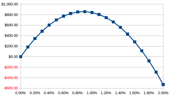
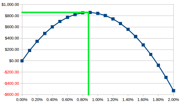
Obviously, using a capital exposure of 0% per trade produces no profits or losses. Risking too much causes the curve to eventually go negative, and there is some maximum somewhere between 0.8% and 1.0%.
Kelly Criterion
We begin with the Kelly Criterion [1], which determines the percentage of an account to risk for any opportunity:
Let:
- $W$ represent win chance/percentage $\left( p = W \right)$
- $b$ represent "profit/loss ratio" $b = {G \over L}$
Then:
$$k = {W - {{1 - W} \over b}}$$
For the previous example:
$$k = \left( {0.42 - {{1 - 0.42} \over { \left( {0.91 \over 0.65} \right) }}} \right) = 0.005714$$
This $k$, is the Kelly Criterion. It represents the percentage of the account to risk per trade.
Now, we are going to make a mistake. Please follow along closely.
Our account size is \$150,000 USD and we wish to risk 0.5714% per trade, so we'll risk \$857.10 USD per trade. We place a limit to buy USDJPY at 120.00 with an initial stop at 119.25, which has a capital exposure of $628.93 USD per lot. We enter 1.36 lots.
This is wrong.
Let's return to the graph from earlier. A capital exposure of \$857.10 is 0.5714% and this falls short of the optimum return on the return curve:
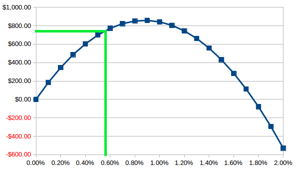
On this particular curve it's fairly close to the top, but clearly is not the optimum. The closer $L$ is to $1.00$, the closer the Kelly Criterion would be to the maximum point.
Sanden Criterion
The Kelly Criterion only applies for for systems which have $L = 1.00$. That is, for systems which have stop losses that are never moved (trailed), never exit a position early, never suffer gap moves, and never incur slippage.
Understand what Kelly Criterion really means: we want to lose $0.5714\%$ of the account value each time we are wrong. Since any individual trade with this system loses 65% of its initial capital exposure on average, we have to further divide 0.005714 by 0.65 to get the actual fraction $f$ of the account value to invest per trade:
$$f = {k \over L} = {0.005714 \over 0.65} = 0.00879$$
This $f$ is the Sanden Criterion. It represents the percentage of the account to invest per trade:
$$Sanden = {Kelly \over L}$$
$$f = {W \over L} - {{ \left( 1 - W \right) } \over G}$$
The Sanden Criterion can be independently derived [2] and determines optimal position sizing:
$$f = {0.42 \over 0.65} - {{ \left( 1 - 0.42 \right) } \over 0.91} = 0.008791$$
Now, we're going to correctly determine position sizing.
Our account size is \$150,000 USD and we wish to invest 0.8791% per trade, so we'll use \$1318.65 USD of capital exposure per trade. We place a limit to buy USDJPY at 120.00 with an initial stop at 119.25, which has a capital exposure of $628.93 USD per lot. We enter 2.10 lots.
This is correct.
The Sanden Criterion applies to all real-life systems which, in general, have $L \neq 1$. In this example, we enter with an initial capital exposure of \$1318.65 USD but on average take 65% of this value when taking a loss, which is \$857.12 . This position sizing maximizes the long-run expectancy of the system.
Sanden Expectancy
Now that we know the correct capital exposure, the percentage of the account to invest in each opportunity, we can plug that back into the account value formula from earlier to determine the expectancy of an individual trade.
We begin with the account value as a function of $f$:
$$A = A_0 \cdot (1 + f \cdot G)^{105} \cdot (1 - f \cdot L)^{145}$$
We'll generalize the formula to use $N \cdot W$ wins and $(1-W) \cdot N$ losses:
$$A = A_0 \cdot (1 + f \cdot G)^{N \cdot W} \cdot (1 - f \cdot L)^{(1-W) \cdot N}$$
To find the percent return, divide both sides by the starting account balance, $A_0$:
$${A \over A_0} = (1 + f \cdot G)^{N \cdot W} \cdot (1 - f \cdot L)^{(1-W) \cdot N}$$
Now, plug in the Sanden Criterion for $f$:
$$f = {W \over L} - {{ \left( 1 - W \right) } \over G}$$
$${A \over A_0} = \left[1 + \left( {{W \over L} - {{ \left( 1 - W \right) } \over G}} \right) \cdot G\right]^{\left(N \cdot W\right)} \cdot \left[1 - \left( {{W \over L} - {{ \left( 1 - W \right) } \over G}} \right) \cdot L\right]^{\left((1-W) \cdot N\right)}$$
Now, to find the per-trade return, raise both sides to the power of $1 \over N$:
$${\left( A \over A_0 \right)}^{1 \over N} = \left[1 + \left( {{W \over L} - {{ \left( 1 - W \right) } \over G}} \right) \cdot G\right]^{{\left(N \cdot W\right)} \over N} \cdot \left[1 - \left( {{W \over L} - {{ \left( 1 - W \right) } \over G}} \right) \cdot L\right]^{{\left((1-W) \cdot N\right)} \over N}$$
Define $E \triangleq {\left( A \over A_0 \right)}^{1 \over N}$ as the Sanden Expectancy of the system.
Simplifying:
$$E = \left( G+L \right) \left( {W \over L} \right)^W \left( {{1-W} \over G} \right)^{ \left( 1-W \right)}$$
$E$ represents the expected value after a single trade. Continuing with our example:
$$E = \left( 0.91+0.65 \right) \left( {0.42 \over 0.65} \right)^{0.42} \left( {{1-0.42} \over 0.91} \right)^{ \left( 1-0.42 \right)} = 1.00002284$$
So, the expected value of our \$150,000 USD account after one trade on our (very questionable) example system at optimal position sizing is $(\$150,000) \cdot 1.00002284\ = \$150003.426$, or on average about $\$3.43$ profit per trade.
Note that if the Sanden Criterion is negative, $f<0$, then this assumes you are taking positions against the system. Therefore, it's probably most reasonable to use $E=1.00$ -- coinciding with a position size of 0, when $f<0$.
Finally, understand that it's possible to have a system with a lower Sanden Criterion that has a larger Sanden Expectancy. The Sanden Criterion as simply a tool to help maximize profitability, whereas the Expectancy represents a system's per-trade profitability at its optimum performance.
Cumulative Expectancy
Given two otherwise identical systems, we'll always want the one that produces more trades per unit time, because that provides more opportunity to compound returns. The Cumulative Expectancy is the total expected return after a given $N$ number of trades. It's just the Sanden Expectancy raised to the power $N$:
$$E_{cumulative} = E^N$$
For example, if $E=1.00002284$, the cumulative expectancy for $N=250$ trades is:
$$E_{cumulative} = \left( 1.00002284 \right)^{250} = 1.005726268$$
or, about 0.57% per month.
When comparing systems it's most useful to compare their Cumulative Expectancy. This takes into account their win rate, average gain, average loss, and number of trades per unit time to arrive at a useful measure of profitability.
--- Chapter 07: ??? ---
lorem ipsum dolor sit amet
--- Chapter 08: Currency Baskets ---
Currency Baskets
Another useful concept is that of a basket, an equally-weighted collection of all of the major crosses for a particular currency. This is different from a currency index -- compare the following:
AUD Index:
$$ AUD = {AUD \over USD} \cdot USD $$
AUD Basket:
$$ AUD = -c_1 {EUR \over AUD} -c_2 {GBP \over AUD} + c_3 {AUD \over NZD} + c_4 {AUD \over USD} + c_5 {AUD \over CAD} + c_6 {AUD \over CHF} + c_7 {AUD \over JPY} $$
First, ignore the coefficients $c_1...c_7$. We'll explain them later. Instead, notice that the AUD Basket is essentially a collection of all of the major AUD-crosses (that is, major pairs containing AUD).
Also note that ${EUR \over AUD}$ and ${GBP \over AUD}$ have negative terms in the equation above. This is because they have AUD on the denominator, so when the value of AUD increases (all else equal), they decrease, and thus are inversely-correlated with the value of AUD. The rest of the crosses have AUD on the numerator, so these are directly correlated, and have positive terms.
Let's pretend that we want to buy the AUD basket. Here are the pairs we would trade:
Short EURAUD
Short GBPAUD
Long AUDNZD
Long AUDUSD
Long AUDCAD
Long AUDCHF
Long AUDJPY
However, it would be wrong to enter the same size trade for each of those pairs. That is, some of those pairs need larger positions and others smaller positions, in order to balance them out.
Each pair has a distributed balancing coefficient, $ c_1...c_7 $ which represents the quantity that should be bought or sold in order to produce a balanced, equally-weighted currency basket. RealFX.co calculates these for you and displays them in real-time, so that you can create and rebalance currency baskets easily. Below, we expound on the details and logic behind these coefficients so that you can calculate them yourself.
Balancing Coefficients
Begin with the profit/loss formula $P$ as a function of price $p$. This represents a trade currently open, with a floating profit/loss:
$$P(p) = S \cdot Ψ \cdot (p - p_0) \cdot {CounterCurrency \over USD}$$
For a 1% increase, $p = 1.01 \cdot p_0$ :
$$P(1.01 \cdot p_0) = S \cdot Ψ \cdot (0.01 \cdot p_0) \cdot {CounterCurrency \over USD}$$
For an 0.01% increase, $p = 1.0001 \cdot p_0$ :
$$P(1.0001 \cdot p_0) = S \cdot Ψ \cdot (0.0001 \cdot p_0) \cdot {CounterCurrency \over USD}$$
And so forth, generalized to $p = (1+\epsilon) \cdot p_0$ :
$$P((1+\epsilon) \cdot p_0) = S \cdot Ψ \cdot (\epsilon \cdot p_0) \cdot {CounterCurrency \over USD}$$
We are taking care to ensure that we measure profit as a function of a percentage change in price. It would be wrong to increase each pair by a constant value; we must raise each pair by a constant percentage instead.
Now, define a multiplicative derivative to measure the profit due to an infinitesimal percentage change:
$${\lim_{\epsilon\to0}} \:\: {{P((1+\epsilon) \cdot p_0) - P(p_0)} \over {\epsilon}}$$
Note that $P(p_0) = 0$, and:
$$P((1+\epsilon) \cdot p_0) = S \cdot Ψ \cdot {{CounterCurrency} \over {USD}} \cdot \left( \epsilon \cdot p_0 \right)$$
Then:
$${\lim_{\epsilon\to0}} \:\: {{P((1+\epsilon) \cdot p_0) - P(p_0)} \over {\epsilon}} = {{ \left[ S \cdot Ψ \cdot {{CC} \over {USD}} \cdot \left( \epsilon \cdot p_0 \right) \right] - \left[ 0 \right]} \over {\epsilon}} = {S \cdot Ψ \cdot {{CounterCurrency} \over {USD}} \cdot p_0 }$$
We now calculate the infinitesimal profit change for EURAUD, noting that $p_0$ is the pair's initial price $(p_0 = {{EUR} \over {AUD}})$:
$$S \cdot Ψ \cdot \left( {{AUD} \over {USD}} \cdot {p_0} \right) = S \cdot Ψ \cdot \left( {{AUD} \over {USD}} \cdot {{EUR} \over {AUD}} \right) = S \cdot Ψ \cdot \left( {{EUR} \over {USD}} \right)$$
Similarly, for all of the pairs in the basket:
EURAUD: $S_{EURAUD} \cdot Ψ \cdot \left( {{AUD} \over {USD}} \cdot {{EUR} \over {AUD}} = {{EUR} \over {USD}} \right)$GBPAUD: $S_{GBPAUD} \cdot Ψ \cdot \left( {{AUD} \over {USD}} \cdot {{GBP} \over {AUD}} = {{GBP} \over {USD}} \right)$AUDNZD: $S_{AUDNZD} \cdot Ψ \cdot \left( {{NZD} \over {USD}} \cdot {{AUD} \over {NZD}} = {{AUD} \over {USD}} \right)$AUDUSD: $S_{AUDUSD} \cdot Ψ \cdot \left( {{USD} \over {USD}} \cdot {{AUD} \over {USD}} = {{AUD} \over {USD}} \right)$AUDCAD: $S_{AUDCAD} \cdot Ψ \cdot \left( {{CAD} \over {USD}} \cdot {{AUD} \over {CAD}} = {{AUD} \over {USD}} \right)$AUDCHF: $S_{AUDCHF} \cdot Ψ \cdot \left( {{CHF} \over {USD}} \cdot {{AUD} \over {CHF}} = {{AUD} \over {USD}} \right)$AUDJPY: $S_{AUDJPY} \cdot Ψ \cdot \left( {{JPY} \over {USD}} \cdot {{AUD} \over {JPY}} = {{AUD} \over {USD}} \right)$
We have also replaced $S$ with $S_{pair}$ for each pair. These will become our (pair) Balancing Coefficients.
Notice that each of these takes the form:
$$S_{pair} \cdot Ψ \cdot {{ContractCurrency} \over {AccountBaseCurrency}}$$
Since our goal is to create an equally-weighted basket, we want each currency pair in the basket to produce an equivalent profit/loss contribution for an equal percentage change in price.
Next, we set each infinitesimal profit change to Ψ (trust me) units of the account's base currency, and solve for the $S_{pair}$ Balancing Coefficient which produces that profit/loss contribution:
$$S_{pair} \cdot Ψ \cdot {{ContractCurrency} \over {AccountBaseCurrency}} = Ψ$$
Solving for $S_{pair}$ :
$$S_{pair} = {AccountBaseCurrency \over ContractCurrency}$$
Therefore, in a currency basket, all pairs with the same Contract-Currency (not Counter-Currency) will have an equal position size ($S$) in the basket, because they will all have the same Balancing Coefficient ($S_{pair}$).
We chose to set each infinitesimal profit change to Ψ in order to produce a "unit-sized" contribution. This can be seen by substituting $S_{pair}$ back into the Profit/Loss formula. Start with:
$$P(p) = S \cdot Ψ \cdot (p - p_0) \cdot {CounterCurrency \over AccountBaseCurrency}$$
Then, Let:
- $S = S_{pair} = {AccountBaseCurrency \over ContractCurrency}$
- $p_0 = {ContractCurrency \over CounterCurrency}$
- $p = 1.01 \cdot p_0$, which represents a 1% price increase
This gives:
Simplifying:
$$P(p) = {{ \left( {AccountBaseCurrency \over ContractCurrency} \right)} \cdot {\left( {CounterCurrency} \over {AccountBaseCurrency} \right)}} \cdot \left( {ContractCurrency \over CounterCurrency} \right) \cdot Ψ \cdot (1.01) $$
$$P(p) = Ψ \cdot (1.01) $$
So, by choosing $S_{pair}$ in this way, a 1% change in price produces profits of $\left( 1\% \cdot Ψ \right)$. In other words a 1-lot-sized position represents a \$100,000 USD investment, and a 1% increase in price would produce \$1000 USD profit -- this is intuitive and convenient, it works for individual pairs as well as baskets, and the logic applies to other Account Base Currencies besides USD.
The final step is to distribute that \$1000 profit across the different pairs in the basket, producing the distributed balancing coefficients $c_1...c_7$ from the basket definition at the beginning of this chapter:
$$c_{pair} = {{S_{pair}} \over {7}} = {{\left( {AccountBaseCurrency} \over {ContractCurrency} \right)} \over 7}$$
Where $7$ represents the number of pairs in the basket.
We can now complete our example for buying the AUD basket:
Short EURAUD
Short GBPAUD
Long AUDNZD
Long AUDUSD
Long AUDCAD
Long AUDCHF
Long AUDJPY
We need these relevant USD-crosses to calculate the Balancing Coefficients:
EURUSD = 1.0619
GBPUSD = 1.2457
AUDUSD = 0.7673
Which are:
S_EURAUD = 1/(EUR/USD) = 1/(1.0619) = 0.94171
S_GBPAUD = 1/(GBP/USD) = 1/(1.2457) = 0.80276
S_AUDNZD = 1/(AUD/USD) = 1/(0.7673) = 1.30327
S_AUDUSD = 1/(AUD/USD) = 1/(0.7673) = 1.30327
S_AUDCAD = 1/(AUD/USD) = 1/(0.7673) = 1.30327
S_AUDCHF = 1/(AUD/USD) = 1/(0.7673) = 1.30327
S_AUDJPY = 1/(AUD/USD) = 1/(0.7673) = 1.30327

c_EURAUD = (0.94171 / 7) = 0.13453
c_GBPAUD = (0.80276 / 7) = 0.11468
c_AUDNZD = (1.30327 / 7) = 0.18618
c_AUDUSD = (1.30327 / 7) = 0.18618
c_AUDCAD = (1.30327 / 7) = 0.18618
c_AUDCHF = (1.30327 / 7) = 0.18618
c_AUDJPY = (1.30327 / 7) = 0.18618
We now have the Distributed Balancing Coefficients, and can multiply by our desired basket size.
For example, if we want an AUD basket that represents \$250000 USD, a 1% move will produce \$2500 in profit or loss. 250000 is 2.5 lots (250000/Ψ); we've essentially reduced this basket to a "normal" contract with Counter-Currency equal to the account's base currency.
Finally, build this 2.5-lot position from its pairs:
Basket Value: $250,000 USD
Profit/Loss for 1% change in basket value: $250,000 * 1% = $2500
Lots: 2.5 (250000 / Ψ)

#--- AUD basket composition for $250,000-USD value ---
EURAUD: 2.5  * -0.13453    =    short 0.34 lots
GBPAUD: 2.5  * -0.11468    =    short 0.29 lots
AUDNZD: 2.5  *  0.18618    =     long 0.47 lots
AUDUSD: 2.5  *  0.18618    =     long 0.47 lots
AUDCAD: 2.5  *  0.18618    =     long 0.47 lots
AUDCHF: 2.5  *  0.18618    =     long 0.47 lots
AUDJPY: 2.5  *  0.18618    =     long 0.47 lots
And this completes the composition of the AUD basket. Note that we've deliberately ignored significant figures throughout this document in order to ensure that the calculations are clear.
RealFX.co provides a calculator to easily determine the correct sizing for any basket of any size.
Rebalancing
Since the balancing coefficients described above depend on the current exchange rates, they are constantly changing. Therefore, a currency basket should be rebalanced periodically to return it to equal weighting.
The more pairs that a basket contains, the more often it needs to be rebalanced. It's recommended to rebalance a basket before its value changes by 5%, and perhaps every 2-3%. There is some risk that a basket will not behave in the ideal fashion due to rapid changes in the value of its underlying pairs which prevents you from rebalancing quickly enough, but in practice our experience has been that rebalancing weekly provides adequate behavior to usually produce the expected profit/loss within a 10% margin of error.
--- Chapter 09: Geomean Indexes ---
In the previous chapter we introduced baskets and mentioned that they need to be periodically rebalanced in order to maintain correct proportions. As such, one cannot simply construct a basket of a currency and then plot the price chart of that basket. Using the basket proportions which are correct today wouldn't produce correct pricing a year ago, and vice-versa.
This is a problem that can be solved using a Geomean Index. It represents the value of a continuously-rebalanced basket.
$$AUD = \left[ { \left( {EUR \over AUD} \right)^{-{1 \over 8}} \cdot { \left( GBP \over AUD \right)}^{-{1 \over 8}} \cdot { \left( AUD \over AUD \right) }^{1 \over 8} \cdot { \left( AUD \over NZD \right) }^{1 \over 8} \cdot { \left( AUD \over USD \right) }^{1 \over 8} \cdot { \left( AUD \over CAD \right) }^{1 \over 8} \cdot { \left( AUD \over CHF \right) }^{1 \over 8} \cdot { \left( AUD \over JPY \right) }^{1 \over 8} } \right]$$
This is a geometric mean. The exponents for $\left( {EUR \over AUD} \right)$ and $\left( {GBP \over AUD} \right)$ are negative since they represent $\left( {AUD \over EUR} \right)$ and $\left( {AUD \over GBP} \right)$.
Note that this includes $\left( {AUD \over AUD} \right)^{1 \over 8} = 1$. We'll carry it along for now for demonstrative purposes.
Sanity Check
For any index to be correct, it must reduce to the correct pair when a ratio is taken. For example, irrespective of how we define an AUD index and NZD index, it must reduce to AUDNZD when the first is divided by the second.
This property is true for the Rational Index described in Chapter 1:
$$AUD_{index} \triangleq \left( {AUD \over USD} \right) \cdot USD_{index}$$ $$NZD_{index} \triangleq \left( {NZD \over USD} \right) \cdot USD_{index}$$ $${AUD_{index} \over NZD_{index}} = {{ \left( {AUD \over USD} \right) \cdot USD_{index}} \over { \left( {NZD \over USD} \right) \cdot USD_{index}}} = {AUD \over NZD}$$
It's also true for the Geomean Index as well:
$$AUD_{index} \triangleq \left[ { \left( {EUR \over AUD} \right)^{-{1 \over 8}} \cdot { \left( GBP \over AUD \right)}^{-{1 \over 8}} \cdot { \left( AUD \over AUD \right) }^{1 \over 8} \cdot { \left( AUD \over NZD \right) }^{1 \over 8} \cdot { \left( AUD \over USD \right) }^{1 \over 8} \cdot { \left( AUD \over CAD \right) }^{1 \over 8} \cdot { \left( AUD \over CHF \right) }^{1 \over 8} \cdot { \left( AUD \over JPY \right) }^{1 \over 8} } \right]$$ $$NZD_{index} \triangleq \left[ { \left( {EUR \over NZD} \right)^{-{1 \over 8}} \cdot { \left( GBP \over NZD \right)}^{-{1 \over 8}} \cdot { \left( AUD \over NZD \right) }^{-{1 \over 8}} \cdot { \left( NZD \over NZD \right) }^{1 \over 8} \cdot { \left( NZD \over USD \right) }^{1 \over 8} \cdot { \left( NZD \over CAD \right) }^{1 \over 8} \cdot { \left( NZD \over CHF \right) }^{1 \over 8} \cdot { \left( NZD \over JPY \right) }^{1 \over 8} } \right]$$
$${AUD_{index} \over NZD_{index}} = { \left[ {{ \left( {EUR \over AUD} \right)^{-{1 \over 8}} \cdot { \left( GBP \over AUD \right)}^{-{1 \over 8}} \cdot { \left( AUD \over AUD \right) }^{1 \over 8} \cdot { \left( AUD \over NZD \right) }^{1 \over 8} \cdot { \left( AUD \over USD \right) }^{1 \over 8} \cdot { \left( AUD \over CAD \right) }^{1 \over 8} \cdot { \left( AUD \over CHF \right) }^{1 \over 8} \cdot { \left( AUD \over JPY \right) }^{1 \over 8} }} \right] \over { \left[ { \left( {EUR \over NZD} \right)^{-{1 \over 8}} \cdot { \left( GBP \over NZD \right)}^{-{1 \over 8}} \cdot { \left( AUD \over NZD \right) }^{-{1 \over 8}} \cdot { \left( NZD \over NZD \right) }^{1 \over 8} \cdot { \left( NZD \over USD \right) }^{1 \over 8} \cdot { \left( NZD \over CAD \right) }^{1 \over 8} \cdot { \left( NZD \over CHF \right) }^{1 \over 8} \cdot { \left( NZD \over JPY \right) }^{1 \over 8} } \right] }}$$
$${AUD_{index} \over NZD_{index}} = { \left( {\left( {EUR \over AUD} \right)^{-{1 \over 8}} \over \left( {EUR \over NZD} \right)^{-{1 \over 8}}} \right) \cdot \left( {\left( {GBP \over AUD} \right)^{-{1 \over 8}} \over \left( {GBP \over NZD} \right)^{-{1 \over 8}}} \right) \cdot \left( {\left( {AUD \over AUD} \right)^{1 \over 8} \over \left( {AUD \over NZD} \right)^{-{1 \over 8}}} \right) \cdot \left( {\left( {AUD \over NZD} \right)^{1 \over 8} \over \left( {NZD \over NZD} \right)^{1 \over 8}} \right) \cdot \left( {\left( {AUD \over USD} \right)^{1 \over 8} \over \left( {NZD \over USD} \right)^{1 \over 8}} \right) \cdot \left( {\left( {AUD \over CAD} \right)^{1 \over 8} \over \left( {NZD \over CAD} \right)^{1 \over 8}} \right) \cdot \left( {\left( {AUD \over CHF} \right)^{1 \over 8} \over \left( {NZD \over CHF} \right)^{1 \over 8}} \right) \cdot \left( {\left( {AUD \over JPY} \right)^{1 \over 8} \over \left( {NZD \over JPY} \right)^{1 \over 8}} \right) }$$
$${AUD_{index} \over NZD_{index}} = \left[ {{ \left( {AUD \over NZD} \right) }^{1 \over 8}} \cdot {{ \left( {AUD \over NZD} \right) }^{1 \over 8}} \cdot {{ \left( {AUD \over NZD} \right) }^{1 \over 8}} \cdot {{ \left( {AUD \over NZD} \right) }^{1 \over 8}} \cdot {{ \left( {AUD \over NZD} \right) }^{1 \over 8}} \cdot {{ \left( {AUD \over NZD} \right) }^{1 \over 8}} \cdot {{ \left( {AUD \over NZD} \right) }^{1 \over 8}} \cdot {{ \left( {AUD \over NZD} \right) }^{1 \over 8}} \right] = {AUD \over NZD}$$
Rational Geomean Index
We can now combine the concepts of the Rational Index and Geomean Index to form the Rational Geomean.
In Chapter 1, we defined the USD index to be the trade-weighted index published by the Federal Reserve. This is not wrong and in fact it's still our preferred method for obtaining a USD index. However, this is not the only way to obtain a USD index; we can use a Geomean Index for USD, and then obtain the Geomean Rational index for other currencies from their USD-cross exchange rates.
For example:
$$USD_{index} \triangleq \left[ { \left( {EUR \over USD} \right)^{-{1 \over 8}} \cdot { \left( GBP \over USD \right)}^{-{1 \over 8}} \cdot { \left( AUD \over USD \right) }^{-{1 \over 8}} \cdot { \left( NZD \over USD \right) }^{-{1 \over 8}} \cdot { \left( USD \over CAD \right) }^{1 \over 8} \cdot { \left( USD \over CHF \right) }^{1 \over 8} \cdot { \left( USD \over JPY \right) }^{1 \over 8} } \right]$$
$$AUD_{index} \triangleq \left( {AUD \over USD} \right) \cdot USD_{index}$$
In this case, we're using a USD Geomean Index and then using it to produce the AUD Geomean Rational Index (rather than using an AUD Geomean Index).